Introduction to Machine Learning
How Models Work
Machine learning works in a similar way to identify the patterns from historical data set and use those patterns to make predictions for future decesions. Decision Tree is the basic building blcok for data science models.
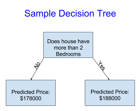
In the example provided in Kaggle course, it uses data to divide houses into two groups and then determine the predicted price in each group.
Fitting/Training model: capture patterns from data
Training data: the data used to fit the model
Leaf: the point at the bottom of Decision Tree where making a prediction
import pandas as pd

# Path of the file to read
iowa_file_path = '../input/home-data-for-ml-course/train.csv'

# Fill in the line below to read the file into a variable home_data
home_data = pd.read_csv(iowa_file_path)

# Print summary statistics in next line
home_data.describe()

# Print all columns of the dataset
home_data.columns

# dropna drops missing values (think of na as "not available")
home_data = home_data.dropna(axis=0)
When dataset had too many variables, we may want to pick few or prioritize variables. The Pandas Micro-Course covers how to select a subset of data in more depth. Two starting approaches:
- Dot notation: use to select the “prediction target”. The single column is stored in a Series.
- Chosing “Features”: use to select the “features”. The columns are inputted into our model and later to make predictions.
# Prediction target
y = home_data.Price

# Chosing features
home_features = ['Rooms', 'Bathroom', 'Landsize', 'Lattitude', 'Longtitude']
X = home_data[home_features]
Steps to build and use the model
- Define: what type of model will it be? Decision tree, etc.
- Fit: capture patterns from provided data. Heart of modeling.
- Predict
- Evaluate: determine the accuracy of the model’s predition.
An example of degining a decision tree model with scikit-learn and fitting it with the features and target variable.
Machine learning models here allow some randomness in model training random_state
from sklearn.tree import DecisionTreeRegressor

# Define model. Specify a number for random_state to ensure same results each run
home_model = DecisionTreeRegressor(random_state=1)

# Fit model
home_model.fit(X, y)

print("Making predictions for the following 5 houses:")
print(X.head())
print("The predictions are")
print(home_model.predict(X.head()))
Model Validation
The relevant measure of model quality is predictive accutacy. The prediction error for each data is:
error = actual - predicted
Mean Absolute Error (MAE): absolute value of each error. On average, our predictions are off by about X
from sklearn.metrics import mean_absolute_error

predicted_home_prices = home_model.predict(X)
mean_absolute_error(y, predicted_home_prices)
Problem with In-sample score: we used a single “sample” of houses for both building the model and evaluating it. Since the pattern was derived from the training data, the model will appear accurate in the training data. However, if the pattern doesn’t hold when the model sees new data, the model would be very inaccurate when used in practice.
Solution - validation data: since model’s practical value come form making predictions on new data, we measure performance on data that wasn’t used to build the model. The most straightforward way to do this is to exclude some data from the model-building process and then use those to test the model’s accuracy on data it hasn’t seen before.
from sklearn.model_selection import train_test_split

# split data into training and validation data, for both features and target
# The split is based on a random number generator. Supplying a numeric value to
# the random_state argument guarantees we get the same split every time we
# run this script.
train_X, val_X, train_y, val_y = train_test_split(X, y, random_state = 0)
# Define model
hoome_model = DecisionTreeRegressor()
# Fit model
home_model.fit(train_X, train_y)

# get predicted prices on validation data
val_predictions = home_model.predict(val_X)
print(mean_absolute_error(val_y, val_predictions))
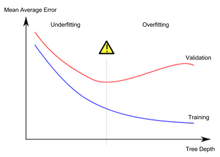
Underfting and Overfitting
Overfitting: capturing spurious patterns that won’t recur in the future, leading to less accurate predictions.
The model matches the training data almost perfectly, but does poorly in validation and other new data. Data is divided amongst many leaves with fewer data samples. Leaves with very few data samples will make preditions that are quite close to those sample’s actual predicted values. However, they may make very unreliable predictions for new data.
Unverfitting: failing to capture relevant patterns, again leading to less accurate predictions.
The model fails to capture important distinctions and patterns in the data, so it performs poorly even in training data.
Random Forests
The random forest uses many trees, and it makes a prediction by averaging the predictions of each component tree. It generally has much better predictive accuracy than a single decision tree and it works well with default parameters.
from sklearn.ensemble import RandomForestRegressor
from sklearn.metrics import mean_absolute_error

forest_model = RandomForestRegressor(random_state=1)
forest_model.fit(train_X, train_y)
melb_preds = forest_model.predict(val_X)
print(mean_absolute_error(val_y, melb_preds))
Data Cleaning
Missing Values
- Drop columns with missing values
# Get names of columns with missing values
cols_with_missing = [col for col in X_train.columns
                     if X_train[col].isnull().any()]

# Drop columns in training and validation data
reduced_X_train = X_train.drop(cols_with_missing, axis=1)
reduced_X_valid = X_valid.drop(cols_with_missing, axis=1)

print("MAE from Approach 1 (Drop columns with missing values):")
print(score_dataset(reduced_X_train, reduced_X_valid, y_train, y_valid))
- Imputation: fills in the missing values with some number.
from sklearn.impute import SimpleImputer

# Imputation
my_imputer = SimpleImputer()
imputed_X_train = pd.DataFrame(my_imputer.fit_transform(X_train))
imputed_X_valid = pd.DataFrame(my_imputer.transform(X_valid))

# Imputation removed column names; put them back
imputed_X_train.columns = X_train.columns
imputed_X_valid.columns = X_valid.columns

print("MAE from Approach 2 (Imputation):")
print(score_dataset(imputed_X_train, imputed_X_valid, y_train, y_valid))
- An extension to imputation: based on imputation, add indication on which values were originally missing.
# Make copy to avoid changing original data (when imputing)
X_train_plus = X_train.copy()
X_valid_plus = X_valid.copy()

# Make new columns indicating what will be imputed
for col in cols_with_missing:
    X_train_plus[col + '_was_missing'] = X_train_plus[col].isnull()
    X_valid_plus[col + '_was_missing'] = X_valid_plus[col].isnull()

# Imputation
my_imputer = SimpleImputer()
imputed_X_train_plus = pd.DataFrame(my_imputer.fit_transform(X_train_plus))
imputed_X_valid_plus = pd.DataFrame(my_imputer.transform(X_valid_plus))

# Imputation removed column names; put them back
imputed_X_train_plus.columns = X_train_plus.columns
imputed_X_valid_plus.columns = X_valid_plus.columns

print("MAE from Approach 3 (An Extension to Imputation):")
print(score_dataset(imputed_X_train_plus, imputed_X_valid_plus, y_train, y_valid))
Categotical Variables
- Drop categorical variables
# Get list of categorical variables
s = (X_train.dtypes == 'object')
object_cols = list(s[s].index)

print("Categorical variables:")
print(object_cols)

drop_X_train = X_train.select_dtypes(exclude=['object'])
drop_X_valid = X_valid.select_dtypes(exclude=['object'])

print("MAE from Approach 1 (Drop categorical variables):")
print(score_dataset(drop_X_train, drop_X_valid, y_train, y_valid))
- Label encoding: assign each unique value to a different integer.
from sklearn.preprocessing import LabelEncoder

# Make copy to avoid changing original data
label_X_train = X_train.copy()
label_X_valid = X_valid.copy()

# Apply label encoder to each column with categorical data
label_encoder = LabelEncoder()
for col in object_cols:
    label_X_train[col] = label_encoder.fit_transform(X_train[col])
    label_X_valid[col] = label_encoder.transform(X_valid[col])

print("MAE from Approach 2 (Label Encoding):")
print(score_dataset(label_X_train, label_X_valid, y_train, y_valid))
- One-Hot encoding: in contrast to label encoding, it does not assume an ordering of the categories. This is expected to work well if there is no clear ordering in the categorical data. Categorical variables are referred as nominal variables without an intrinsic ranking.
from sklearn.preprocessing import OneHotEncoder

# Apply one-hot encoder to each column with categorical data
OH_encoder = OneHotEncoder(handle_unknown='ignore', sparse=False)
OH_cols_train = pd.DataFrame(OH_encoder.fit_transform(X_train[object_cols]))
OH_cols_valid = pd.DataFrame(OH_encoder.transform(X_valid[object_cols]))

# One-hot encoding removed index; put it back
OH_cols_train.index = X_train.index
OH_cols_valid.index = X_valid.index

# Remove categorical columns (will replace with one-hot encoding)
num_X_train = X_train.drop(object_cols, axis=1)
num_X_valid = X_valid.drop(object_cols, axis=1)

# Add one-hot encoded columns to numerical features
OH_X_train = pd.concat([num_X_train, OH_cols_train], axis=1)
OH_X_valid = pd.concat([num_X_valid, OH_cols_valid], axis=1)

print("MAE from Approach 3 (One-Hot Encoding):")
print(score_dataset(OH_X_train, OH_X_valid, y_train, y_valid))
Pipelines
Pipelines are a simple way to keep data preprocessing and modeling code organized.
Benefits:
- Cleaner code
- Fewer bugs
- Easier to productionize
- More options for model validation
Steps:
- Define preprocessing steps:
- imputes missing values in numerical data
- imputed missing values and applies a one-hot encoding to categotical data
from sklearn.compose import ColumnTransformer
from sklearn.pipeline import Pipeline
from sklearn.impute import SimpleImputer
from sklearn.preprocessing import OneHotEncoder

# Preprocessing for numerical data
numerical_transformer = SimpleImputer(strategy='constant')

# Preprocessing for categorical data
categorical_transformer = Pipeline(steps=[
    ('imputer', SimpleImputer(strategy='most_frequent')),
    ('onehot', OneHotEncoder(handle_unknown='ignore'))
])

# Bundle preprocessing for numerical and categorical data
preprocessor = ColumnTransformer(
    transformers=[
        ('num', numerical_transformer, numerical_cols),
        ('cat', categorical_transformer, categorical_cols)
    ])
- Define the model
from sklearn.ensemble import RandomForestRegressor

model = RandomForestRegressor(n_estimators=100, random_state=0)
- Create and evaluate the pipeline
from sklearn.metrics import mean_absolute_error

# Bundle preprocessing and modeling code in a pipeline
my_pipeline = Pipeline(steps=[('preprocessor', preprocessor),
                              ('model', model)
                             ])

# Preprocessing of training data, fit model
my_pipeline.fit(X_train, y_train)

# Preprocessing of validation data, get predictions
preds = my_pipeline.predict(X_valid)

# Evaluate the model
score = mean_absolute_error(y_valid, preds)
print('MAE:', score)
Cross-Validation
Run modeling process on different subsets of the data to get multiple measures of model quality.
Cross-validation gives a more accurate measure of model quality, which is especially important if in need to make a lot of modeling decisions.
Therefore:
- For small datasets, where extra computational burden isn’t a big deal, run cross-validation
- For larger datasets, a single validation set is sufficient. Code will run faster, and there is enough data that there’s little need to re-use some of it for holdout.
from sklearn.ensemble import RandomForestRegressor
from sklearn.pipeline import Pipeline
from sklearn.impute import SimpleImputer

my_pipeline = Pipeline(steps=[('preprocessor', SimpleImputer()),
                              ('model', RandomForestRegressor(n_estimators=50,
                                                              random_state=0))
                             ])

from sklearn.model_selection import cross_val_score

# Multiply by -1 since sklearn calculates *negative* MAE
scores = -1 * cross_val_score(my_pipeline, X, y,
                              cv=5,
                              scoring='neg_mean_absolute_error')

print("MAE scores:\n", scores)
XGBoost
Gradient boosting goes through cycles to iteratively add models into an ensemble. It begins by initializing the enselmble with a single model with naive prediction. Then we start the cycle:
- Use the current ensemble to generate predictions for each observation in the dataset.
- These predictions are used to calculate a loss function.
- Use loss function to fit a new model that will be added to the ensemblbe.
- Finally, add the new model to ensemble.
from xgboost import XGBRegressor

my_model = XGBRegressor(n_estimators=500, learning_rate=0.05, n_jobs=4))
my_model.fit(X_train, y_train,
            early_stopping_rounds=5,
            eval_set=[(X_valid, y_valid)],
            verbose=False)

from sklearn.metrics import mean_absolute_error

predictions = my_model.predict(X_valid)
print("Mean Absolute Error: " + str(mean_absolute_error(predictions, y_valid)))
Data Leakage
Data leakage happens when training data contains information about the target but similar data will not be available when the model is used for prediction. This lead to high performance on the training set, but the model will perform poorly in production.
- Target leakage: occurs when predictors include data that will not be available at the time making predictions.
- Train-test contamination: occurs when not distinguish training data from validation data.
from sklearn.pipeline import make_pipeline
from sklearn.ensemble import RandomForestClassifier
from sklearn.model_selection import cross_val_score

# Since there is no preprocessing, we don't need a pipeline (used anyway as best practice!)
my_pipeline = make_pipeline(RandomForestClassifier(n_estimators=100))
cv_scores = cross_val_score(my_pipeline, X, y,
                            cv=5,
                            scoring='accuracy')

print("Cross-validation accuracy: %f" % cv_scores.mean())

expenditures_cardholders = X.expenditure[y]
expenditures_noncardholders = X.expenditure[~y]

print('Fraction of those who did not receive a card and had no expenditures: %.2f' \
      %((expenditures_noncardholders == 0).mean()))
print('Fraction of those who received a card and had no expenditures: %.2f' \
      %(( expenditures_cardholders == 0).mean()))

# Drop leaky predictors from dataset
potential_leaks = ['expenditure', 'share', 'active', 'majorcards']
X2 = X.drop(potential_leaks, axis=1)

# Evaluate the model with leaky predictors removed
cv_scores = cross_val_score(my_pipeline, X2, y,
                            cv=5,
                            scoring='accuracy')

print("Cross-val accuracy: %f" % cv_scores.mean())